MaxK-GNN

intro

GCN，传统的 GCN 加速通过将图形特征矩阵（ X ）与密集的小权重矩阵（ W ）相乘，然后通过稀疏-密集矩阵矩阵乘法（SpMM）将结果输出与高度稀疏的不规则邻接矩阵（ A ）相乘。

Achievement

algorithmic optimization and hardware-level enhancement

graph reordering, run-time community detection,graph partitioning
workload balancing and efficient hardware mapping

challenges

accelerators based on ASIC/FPGA instead of GPU
GPU ...far from meeting performance limits
- Why
  - Memory Traffic Challenges in GPU-based Frameworks
    - row-wise multiplication
    - still requires a substantial number of global memory transactions to access the input feature matrix
    - linear scaling with $d i m_{o r i g i n}$ and $n n z$
  - Algorithmic Limitations and Resource Waste: This architecture-oblivious workflow consistently results in inefficient hardware utilization.

Proposed Research

code
- pytorch frontend
- customizing the MaxK nonlinearity to select the top-k⁢t⁢h element for each node embedding
  - some sample technique?
- SpGEMM/SSpMM kernel
Node-Balanced Feature Dimension Reduction through MaxK Nonlinearity
- 有损优化？
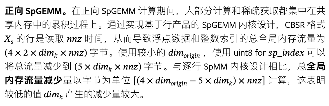
Compressed Balanced Sparse Row (CBSR) format
Coalescing Enhanced Forward Computation with Row-wise Product-Based SpGEMM Kernel
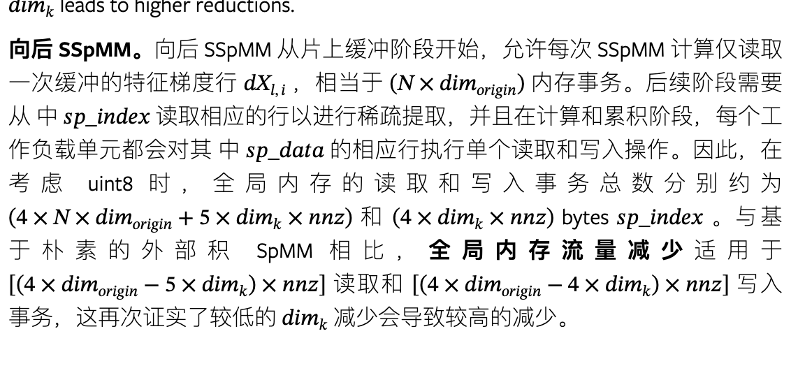
Optimized Backward Computation with Outer Product-Based SSpMM Kernel Design

sidenote

max-k non-leanrity 是不是一个常见的深度学习术语...?

GCN

a graph $G = (𝒱, ℰ, A)$ which contains |𝒱| nodes and |ℰ| edges
- represent as : adjacency matrix A
  - Each non-zero entry A⁢(i,j) corresponds to an edge between i and j.
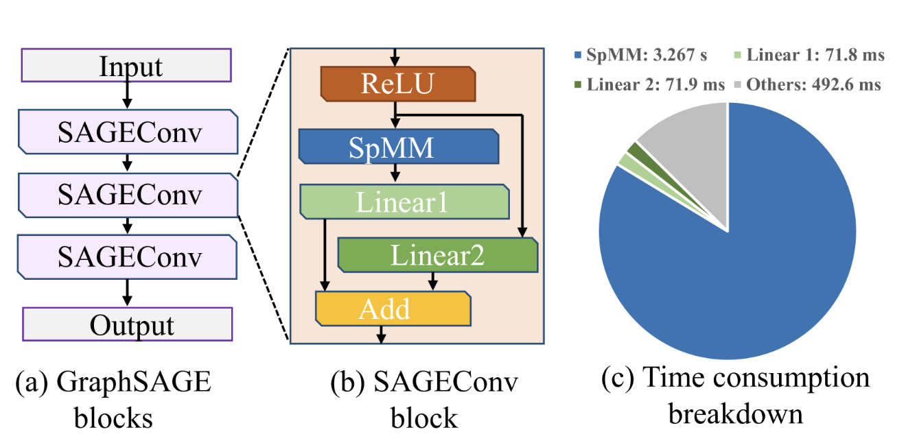
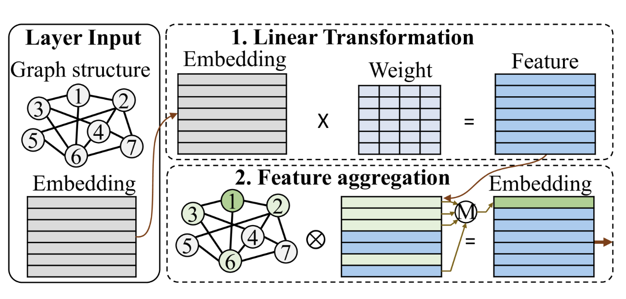
l-th GCNConv layer has 2 stages
- linear $Y^{l} = X^{l} W^{l}$
  - $X^{l} \in R^{| V | \times ？_{l}}$ feature embedding matrix at the $l$ -th layer
  - $W$ weight matrix
- feature aggregation $X^{l + 1} = σ (A^{'} Y^{l})$ 【这应该是卷积步骤？不确定】
  - $A^{'} \in R^{| v | \times | v |}$ normalized and regularized adjacency matrix
  - $σ$ activation function, typically element-wise ReLU

GNN Acceleration

PyTorch Geometric (PyG)...utilize message-passing primitives such as scatter and reduce for GNN training on GPUs and FPGA overlays
- memory and storage overheads
GPU and FPGA acceleration frameworks... uses warp-level partitioning for distributed neighborhood workload
- imbalance...
- MergePath addresses SpMM workload imbalance with a binary search algorithm, but its efficacy decreases with feature dimensions over 128
graph neighborhood and boundary sampling ⇒ fail to address the SpMM bottleneck
specialized hardware

Introducing Sparsity in GNN Training

Dropout: ... challenging to leverage in an system/hardware design.
Weight Sparsification
- train-and-prune and sparse training
- 这个llm里大概也用...
adjusting the ReLU threshold can induce greater feature sparsity
- ReLU的0区域就相当于不要某个神经元了，记得6.激活函数这八股文里讨论过

MaxK-GNN Dataflow

we introduce the MaxK nonlinearity

我悟了，这里是通过魔改激活函数，达到稀疏权重的效果，很神奇.....
（另外一个sidenote是，先多看看overview DL的八股文，等到IRL看到某个领域的时候作为思维的脚手架很有帮助...

definition

(i) During the forward propagation, MaxK nonlinearity is computed on node-wise feature map to get the maximum $k_{t h}$ element and set the rest to 0.
(ii) During the backward propagation, the feature gradient uses same feature sparsity pattern as induced in forward.

h (x) = m a x - k_{j \in [1, r]} (X \cdot W + b)_{j}

这看起来理论背景很复杂，实现比较（？）简洁，这很符合我的审美...

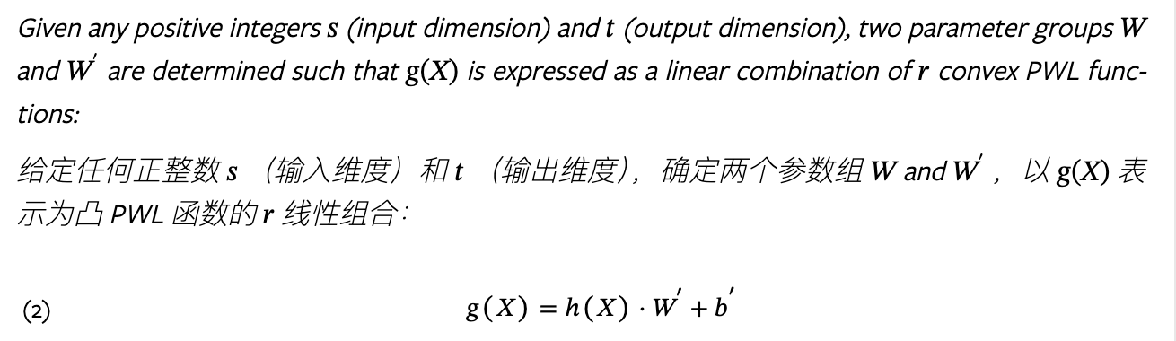
WXb ⇒ 在深度学习里的常见含义
h⁢(X) denotes intermediate feature, which is a piece-wise linear (PWL) function of X
the MaxK nonlinear operator is positioned before the SpMM operator

figa，maxk和relu输入输出维度近似？
figb用MLP拟合 $y = x^{2}$ ，效果上maxk和relu差不多，所以证明它有效？

sidenote：piece-wise linear (PWL) function

原来是分段线性函数的英文，belike relu和高中一些简单的函数题
可视化见下

3.1

应该就是figa的意思？激活函数换了，所以linear层的参数也不一样？

3.2

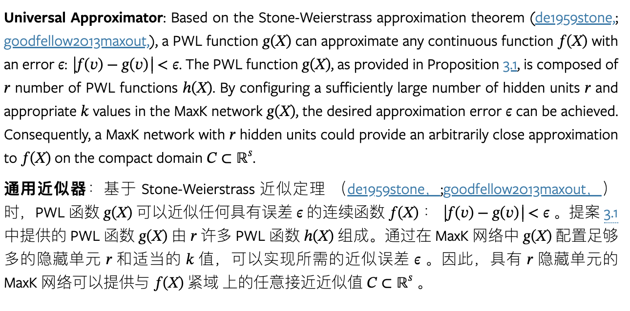
MLP with MaxK Serves as a Universal Approximator. A MaxK network $g (X)$ with $r$ hidden units can approximate any continuous function $f (X)$ on a compact domain $C \subset ℝ^{s}$ with an arbitrarily small approximation error ϵ. In particular, as ϵ→0, it follows that r→∞.

Universal Approximator

MaxK-GNN Training Dataflow

!MaxK-GNN 2024-09-17.excalidraw

GPU System Support for MaxK-GNN

这里进行到实际的cuda kernel的部分了

forward: 特征提取 kenerl设计

!MaxK-GNN 2024-09-17_0.excalidraw

backward

!MaxK-GNN 2024-09-17_1.excalidraw

内存访问合并指什么？有点搞不明白
dimk好像是topk参数，origin是原来的稀疏结果！

memory system

Kernel Profiling

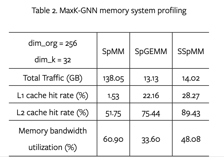
当将原始隐藏维度从 256 减少到 k为 32 时，所提出的 MaxK 非线性和相应的内核支持将总全局内存流量减少了近 90.5% / 89.8%
L1 Cache命中率非常高...

eval

#TODO

按warp提取信息的设计

此计算采用基于行积的 SpGEMM 方案 ( srivastava2020matraptor, ) ，其中 $X l [i, :] = \sum j = 0 J A [i, j] \cdot h (X_{l - 1}) [j, :]$ 。假设密集输出可避免 SpGEMM 设计中通常会遇到的高昂 ESC 开销 ( dalton2015optimizing, ) 。在逐行乘积运算中，左侧行中的每个元素都会与右侧行中对应的元素相乘，然后将结果累加到输出行。此过程使得稀疏化的输出累加能够在片上缓存中进行，与基于全局内存的累加相比，延迟显著降低。

我们使用了一种 warp-level 分区方案。结合片上缓冲机制，该方法可以实现 warp-level 平衡和合并全局内存访问，从而显著提高计算效率

怎么操作？

如图 6 (b) 所示，参与计算的每条边 ei,j 构成一个工作负载单元。在该单元中， ei,j 与稀疏行 s⁢p⁢_⁢d⁢a⁢t⁢aj 相乘，然后在缓冲区 B⁢u⁢fw 中进行累加，该缓冲区的索引为 s⁢p⁢_⁢i⁢n⁢d⁢e⁢xj 。随后，将每个邻接矩阵行 Ar⁢o⁢wi 的工作负载分割为多个边组 ( E⁢G⁢s )。每个 E⁢G 预留一块共享的 ( d⁢i⁢mo⁢r⁢i⁢g⁢i⁢n×4 字节) 空间，作为稀疏累加的中间缓冲区。

首先将每个邻接矩阵行 Ar⁢o⁢wi 的工作负载分割成边缘组 (EG)。为了在计算和累积阶段优化 EG 的执行，我们将隐藏维度集成到 Warp 映射策略中。

在 d⁢i⁢mk≤16 的场景下（如图 6 (b) 中的情况 1 所示），每个标准 Warp 包含 ⌊32/d⁢i⁢mk⌋ 个 EG 工作负载，EG 被限制在同一个 Warp 中，以避免 EG 跨越多个 Warp 时可能发生的内存访问冲突。
相反，如果是 d⁢i⁢mk>16 （如图 6 (b) 中的情况 2 所示），EG 由单个 Warp 迭代执行处理。每个 EG 的执行由相应的 Warp 执行，结果按照 s⁢p⁢_⁢i⁢n⁢d⁢e⁢x 中的索引聚合到共享内存缓冲区中的相应位置。

以图里为例，32/3 = 10，但似乎图里只用了6个，从何理解呢？

在下一阶段（图 6 中的第 2 阶段），来自每个共享内存缓冲区 B⁢u⁢fw 的数据将以原子方式累积到全局内存中其对应的 Xl 输出中。由于共享内存缓冲区和输出嵌入 ( d⁢i⁢mo⁢r⁢i⁢g⁢i⁢n ) 的维度相同，因此保留了自然 Warp 的线程组织方式，每个 Warp 循环处理单行数据，从而确保了高效且合并的计算结构。